Datanami
 EnterpriseAI
 HPCwire Japan
 QCwire
 HPC & AI Wall Street
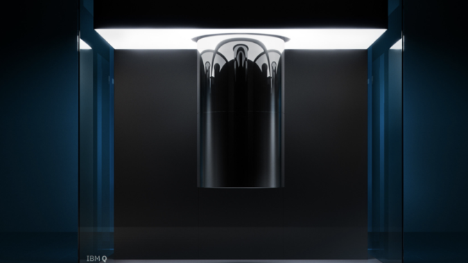
IBM this week announced it had achieved its highest Quantum Volume number to date at the American Physical Society (APS) March meeting being held in Boston. What’s Quantum Volume, you ask? Broadly, it’s a ‘holistic measure’ introduced by IBM in a paper last November that’s intended to characterize gate-based quantum computers, regardless of their underlying technology (semiconductor, ion trap, etc.), with a single number. IBM is urging wide adoption of QV by the quantum computing community.
The idea is interesting. The highest QV score so far is 16 which was attained by IBM’s fourth generation 20-qubit IBM Q System One; that’s double the QV of IBM’s 20-qubit IBM Q Network devices. You can see qubit count isn’t the determinant (but it is a factor). Many system-wide facets – gate error rates, decoherence times, qubit connectivity, operating software efficiency, and more – are effectively baked into the measure. In the paper, IBM likens QV to LINPACK for its ability to compare diverse systems.
IBM has laid out a roadmap in which it believes it can roughly double QVs every year. This rate of progress, argues IBM, will produce quantum advantage – which IBM defines as “a quantum computation is either hundreds or thousands of times faster than a classical computation, or needs a smaller fraction of the memory required by a classical computer, or makes something possible that simply isn’t possible now with a classical computer” – in the 2020s.
Addison Snell, CEO, Intersect360 Research noted, “Quantum volume is an interesting metric for tracking progress toward the ability to leverage quantum computing in ways that would be impractical for conventional supercomputers. With the different approaches to quantum computing, it is difficult to compare this achievement across the industry, but it is nevertheless a compelling statistic.”
There’s a lot to unpack here and it’s best done by reading the IBM paper, which isn’t overly long. Bob Sutor, VP, IBM Q Strategy and Ecosystem, and Sarah Sheldon, research staff at IBM T.J. Watson Research Center, briefed HPCwire on QV’s components, use, and relevance to the pursuit of quantum advantage. Before jumping into how Quantum Value is determined, Sutor’s comments on timing and what the magic QV number might be to achieve quantum advantage are interesting.
“We’re not going to go on record saying this or that particular QV number [will produce quantum advantage]. We have now educated hunches based on the different paths that people are taking, that people are taking for chemistry, for AI explorations, for some of the Monte Carlo simulations, and frankly the QV number may be different and probably will be different for each of those. We are certainly on record as saying in the 2020s and we hope in 3-to-5 years,” said Sutor.

The APS meeting served as a broad launchpad for QV with IBM making several presentations on various quantum topics while also seeking to stimulate conversation and urge adoption of QV within the gate-based quantum computing crowd. IBM issued a press release, a more technical blog with data points, and continued promoting the original paper (Validating quantum computers using randomized model circuits) which is freely downloadable. Rigetti has reportedly implemented QV. Noteworthy, QV is not meant for use with adiabatic annealing quantum systems such as D-Wave’s.
A central challenge in quantum computing is the variety of error and system influences that degrade system control and performance. Lacking practical and powerful enough error correction technology, the community has opted for labelling the modern class of quantum computers as noisy intermediate-scale quantum (NISQ) systems. Recognizing this is a situation likely to persist for some time, the IBM paper’s authors[I] do a nice job describing the problem and their approach to measuring performance. Excerpt:
“In these noisy intermediate-scale quantum (NISQ) systems, performance of isolated gates may not predict the behavior of the system. Methods such as randomized benchmarking, state and process tomography, and gateset tomography are valued for measuring the performance of operations on a few qubits, yet they fail to account for errors arising from interactions with spectator qubits. Given a system such as this, whose individual gate operations have been independently calibrated and verified, how do we measure the degree to which the system performs as a general purpose quantum computer? We address this question by introducing a single-number metric, the quantum volume, together with a concrete protocol for measuring it on near-term systems. Similar to how LINPACK is used for comparing diverse classical computers, this metric is not tailored to any particular system, requiring only the ability to implement a universal set of quantum gates.
“The quantum volume protocol we present is strongly linked to gate error rates, and is influenced by underlying qubit connectivity and gate parallelism. It can thus be improved by moving toward the limit in which large numbers of well-controlled, highly coherent, connected, and generically programmable qubits are manipulated within a state-of-the-art circuit rewriting toolchain. High-fidelity state preparation and readout are also necessary. In this work, we evaluate the quantum volume of current IBM Q devices, and corroborate the results with simulations of the same circuits under a depolarizing error model.”
In practice, explained Sheldon, “We generate model circuits which have a specific form where they are sequences of different layers of random entangling gates. The first step is entangling gates between different pairs of qubits on the device. Then we permute the pairing of qubits, into another layer of entangling gates. Each of these layers we call the depth. So if we have three layers, it’s depth3. What we are looking at are circuits we call square circuits with the same number of qubits as the depth in the circuit. Since we are still talking about small enough numbers of qubits that we can simulate these circuits [on classical systems].
“We run an ideal simulation of the circuit and from get a probability distribution of all the possible outcomes. At the end of applying the circuit, the system should be in some state and if we were to measure it we would get a bunch of bit streams, outcomes, with some probabilities. Then we can compare the probabilities from the ideal case to what we actually measured. Based on how close we are to the ideal situation, we say whether or not we were successful. There are details in the paper about how we actually define the success and how we compare the experimental circuits to the ideal circuits. The main point is by doing these model circuits we’re sort of representing a generic quantum algorithm – [we realize] a quantum algorithm doesn’t use random circuits but this is kind of a proxy for that,” she said.
Shown below are some data characterizing IBM systems – IBM Q System One, IBM Q Network systems “Tokyo” and “Poughkeepsie,” and the publicly-available IBM Q Experience system “Tenerife.” As noted in IBM’s blog the performance of a particular quantum computer can be characterized on two levels: metrics associated with the underlying qubits in the chip—what we call the “quantum device”—and overall full-system performance.

“IBM Q System One’s performance is reflected in some of the best/lowest error rates we have ever measured. The average two qubit gate error is less than two percent, and the best gate has less than one percent error rate. Our devices are close to being fundamentally limited by coherence times, which for IBM Q System One averages 73μs,” write Jay Gambetta (IBM Fellow) and Sheldon in the blog. “The mean two-qubit error rate is within a factor of two (x1.68) of the coherence limit, the theoretical limit set by the qubit T1 and T2 (74μs and 69μs on average for IBM Q System One). This indicates that the errors induced by our controls are quite small, and we are achieving close to the best possible qubit fidelities on this device.”

It will be interesting to see how the quantum computing community responds to the CV metric. Back in May when Hyperion Research launched its quantum practice, analyst Bob Sorensen said, “One of the things I’m hoping we can at least play a role in is the idea of thinking about quantum computing benchmarks. Right now, if you read the popular press, and I say ‘IBM’ and the first thing you think of is, yes they have a 50-qubit system. That doesn’t mean much to anybody other than it’s one more qubit than a 49-qubit system. What I am thinking about is asking these people how can we start to characterize across a number of different abstractions and implementations to gain a sense of how we can measure progress.”
IBM has high hopes for Quantum Volume.
Link to release: https://newsroom.ibm.com/2019-03-04-IBM-Achieves-Highest-Quantum-Volume-to-Date-Establishes-Roadmap-for-Reaching-Quantum-Advantage
Link to blog: https://www.ibm.com/blogs/research/2019/03/power-quantum-device/
Link to paper: https://arxiv.org/pdf/1811.12926.pdf
Feature image; IBM Q System One
[i]Validating quantum computers using randomized model circuits, Andrew W. Cross, Lev S. Bishop, Sarah Sheldon, Paul D. Nation, and Jay M. Gambetta IBM T. J. Watson Research Center, https://arxiv.org/pdf/1811.12926.pdf